Recently the ABC had an article that covered the high temperatures for Perth in May from 1897 to current with a chart showing the values over time. I thought it would be fun to use {weatherOz} to recreate this and maybe dig a little deeper.
To start, you will need to install {weatherOz}, which currently is not on CRAN (yet) and {hrbrthemes} from GitHub as it is ahead of the CRAN version.
|
|
Now, the first question I had from reading the article was, “which station in Perth is this”? As that is not clear, we will see what is available from {weatherOz} keeping in mind that we also have Western Australia’s Department of Primary Industries and Regional Development’s (DPIRD) weather stations available to us for later years as well and that the SILO data are derived from BOM.
With that in mind, let’s see what stations are available for Perth.
Finding
This turned out to be more difficult than I expected.
{weatherOz} provides a find_stations_in() function1 that we can use with either an sf object or a bounding box to find stations in a geographic area of interest.
For this post, I have opted to use an sf object that I created by downloading “Greater Capital City Statistical Areas - 2021 - Shapefile” from the Australian Bureau of Statistics (ABS).
|
|
## Linking to GEOS 3.11.0, GDAL 3.5.3, PROJ 9.1.0; sf_use_s2() is TRUE
|
|
## [1] "GCCSA_2021_AUST_GDA2020.dbf"     "GCCSA_2021_AUST_GDA2020.prj"
## [3] "GCCSA_2021_AUST_GDA2020.shp"     "GCCSA_2021_AUST_GDA2020.shx"
## [5] "GCCSA_2021_AUST_GDA2020.xml"     "GCCSA_2021_AUST_SHP_GDA2020.zip"
## [7] "libloc_219_23065bff165f0f8a.rds" "libloc_258_ca82491e8b2446a2.rds"
## [9] "libloc_259_cfca17948badcd1d.rds"
|
|
## Reading layer `GCCSA_2021_AUST_GDA2020' from data source
##   `/private/var/folders/ch/8fqkzddj1kj_qb5ddfdd3p1w0000gn/T/RtmpIouqPz/GCCSA_2021_AUST_GDA2020.shp'
##   using driver `ESRI Shapefile'
## replacing null geometries with empty geometries
## Simple feature collection with 35 features and 10 fields (with 19 geometries empty)
## Geometry type: GEOMETRY
## Dimension:     XY
## Bounding box:  xmin: 96.81695 ymin: -43.7405 xmax: 167.998 ymax: -9.142163
## Geodetic CRS:  GDA2020
|
|
## Simple feature collection with 35 features and 10 fields (with 19 geometries empty)
## Geometry type: GEOMETRY
## Dimension:     XY
## Bounding box:  xmin: 96.81695 ymin: -43.7405 xmax: 167.998 ymax: -9.142163
## Geodetic CRS:  GDA2020
## First 10 features:
##    GCC_CODE21                             GCC_NAME21 CHG_FLAG21 CHG_LBL21
## 1       1GSYD                         Greater Sydney          0 No change
## 2       1RNSW                            Rest of NSW          0 No change
## 3       19499                 No usual address (NSW)          0 No change
## 4       19799  Migratory - Offshore - Shipping (NSW)          0 No change
## 5       2GMEL                      Greater Melbourne          0 No change
## 6       2RVIC                           Rest of Vic.          0 No change
## 7       29499                No usual address (Vic.)          0 No change
## 8       29799 Migratory - Offshore - Shipping (Vic.)          0 No change
## 9       3GBRI                       Greater Brisbane          0 No change
## 10      3RQLD                            Rest of Qld          0 No change
##    STE_CODE21      STE_NAME21 AUS_CODE21 AUS_NAME21  AREASQKM21
## 1           1 New South Wales        AUS  Australia   12368.686
## 2           1 New South Wales        AUS  Australia  788428.973
## 3           1 New South Wales        AUS  Australia          NA
## 4           1 New South Wales        AUS  Australia          NA
## 5           2        Victoria        AUS  Australia    9992.608
## 6           2        Victoria        AUS  Australia  217503.640
## 7           2        Victoria        AUS  Australia          NA
## 8           2        Victoria        AUS  Australia          NA
## 9           3      Queensland        AUS  Australia   15842.007
## 10          3      Queensland        AUS  Australia 1714329.214
##                                               LOCI_URI21
## 1  http://linked.data.gov.au/dataset/asgsed3/GCCSA/1GSYD
## 2  http://linked.data.gov.au/dataset/asgsed3/GCCSA/1RNSW
## 3  http://linked.data.gov.au/dataset/asgsed3/GCCSA/19499
## 4  http://linked.data.gov.au/dataset/asgsed3/GCCSA/19799
## 5  http://linked.data.gov.au/dataset/asgsed3/GCCSA/2GMEL
## 6  http://linked.data.gov.au/dataset/asgsed3/GCCSA/2RVIC
## 7  http://linked.data.gov.au/dataset/asgsed3/GCCSA/29499
## 8  http://linked.data.gov.au/dataset/asgsed3/GCCSA/29799
## 9  http://linked.data.gov.au/dataset/asgsed3/GCCSA/3GBRI
## 10 http://linked.data.gov.au/dataset/asgsed3/GCCSA/3RQLD
##                          geometry
## 1  MULTIPOLYGON (((151.2816 -3...
## 2  MULTIPOLYGON (((159.0623 -3...
## 3              MULTIPOLYGON EMPTY
## 4              MULTIPOLYGON EMPTY
## 5  MULTIPOLYGON (((144.8883 -3...
## 6  MULTIPOLYGON (((146.2929 -3...
## 7              MULTIPOLYGON EMPTY
## 8              MULTIPOLYGON EMPTY
## 9  MULTIPOLYGON (((153.2321 -2...
## 10 MULTIPOLYGON (((142.5314 -1...
|
|
Finding Weather Stations in the Greater Perth Area
With that available, let’s find stations that fall within the greater Perth area as defined by the ABS. As we need API keys to access the data from {weatherOz}, I’ll use {keyring} to safely handle credentials. The query as defined here includes closed stations, since many early records may be from closed stations.
|
|
##
## Attaching package: 'weatherOz'

## The following object is masked from 'package:graphics':
##
##     plot

## The following object is masked from 'package:base':
##
##     plot
|
|
##   station_code station_name           start                 end
##  009000 : 1    Length:89          Min.   :1852-01-01   Min.   :1930-01-01
##  009001 : 1    Class :character   1st Qu.:1910-01-01   1st Qu.:2001-01-01
##  009003 : 1    Mode  :character   Median :1963-01-01   Median :2024-06-09
##  009007 : 1                       Mean   :1954-02-18   Mean   :2011-10-29
##  009009 : 1                       3rd Qu.:1993-01-01   3rd Qu.:2024-06-09
##  009010 : 1                       Max.   :2024-02-22   Max.   :2024-06-09
##  (Other):83
##     latitude        longitude        state               elev_m
##  Min.   :-32.70   Min.   :115.5   Length:89          Min.   :  3.0
##  1st Qu.:-32.22   1st Qu.:115.8   Class :character   1st Qu.: 18.0
##  Median :-32.01   Median :116.0   Mode  :character   Median : 40.0
##  Mean   :-32.07   Mean   :115.9                      Mean   :108.3
##  3rd Qu.:-31.90   3rd Qu.:116.1                      3rd Qu.:209.2
##  Max.   :-31.56   Max.   :116.3                      Max.   :384.0
##                                                      NA's   :7
##     source             status               wmo
##  Length:89          Length:89          Min.   :94602
##  Class :character   Class :character   1st Qu.:94609
##  Mode  :character   Mode  :character   Median :94613
##                                        Mean   :95025
##                                        3rd Qu.:95607
##                                        Max.   :95614
##                                        NA's   :77
This query returns 89 stations, but some are listed with “CAUTION: Do not use these observations”.
Others are from a portable station, which may not be reliable.
Let’s drop these stations.
|
|
Now there are 80 stations that start on 1852-01-01 and run to current.
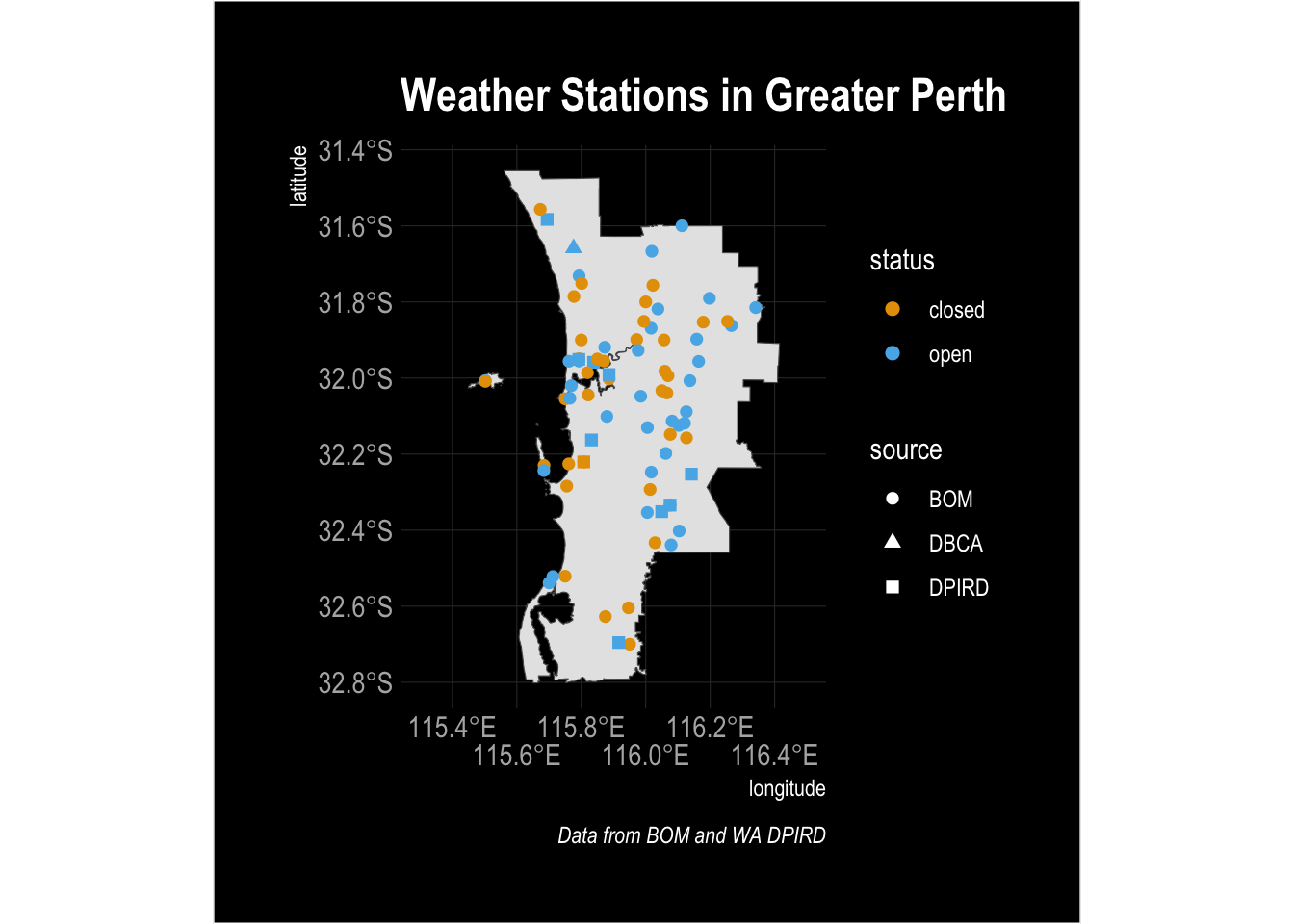
Map the Stations
We can map the stations within the greater Perth area to see where they fall using {ggplot2}, who the station owner is and see if they are open or closed.
I’ve chosen to add a new column to use for the legend to indicate the station data source (owner) in a cleaner fashion using the abbreviation only to save space in the plot legend.
I’ve used the excellent Okabe and Ito palette for this colour scheme as it is colour-blind friendly and easy to see here along with Bob Rudis’s excellent {hrbrthemes}.
Lastly, using {ggdark} I’ve inverted the colour theme to use a dark background with theme_ipsum.
|
|
## Inverted geom defaults of fill and color/colour.
## To change them back, use invert_geom_defaults().
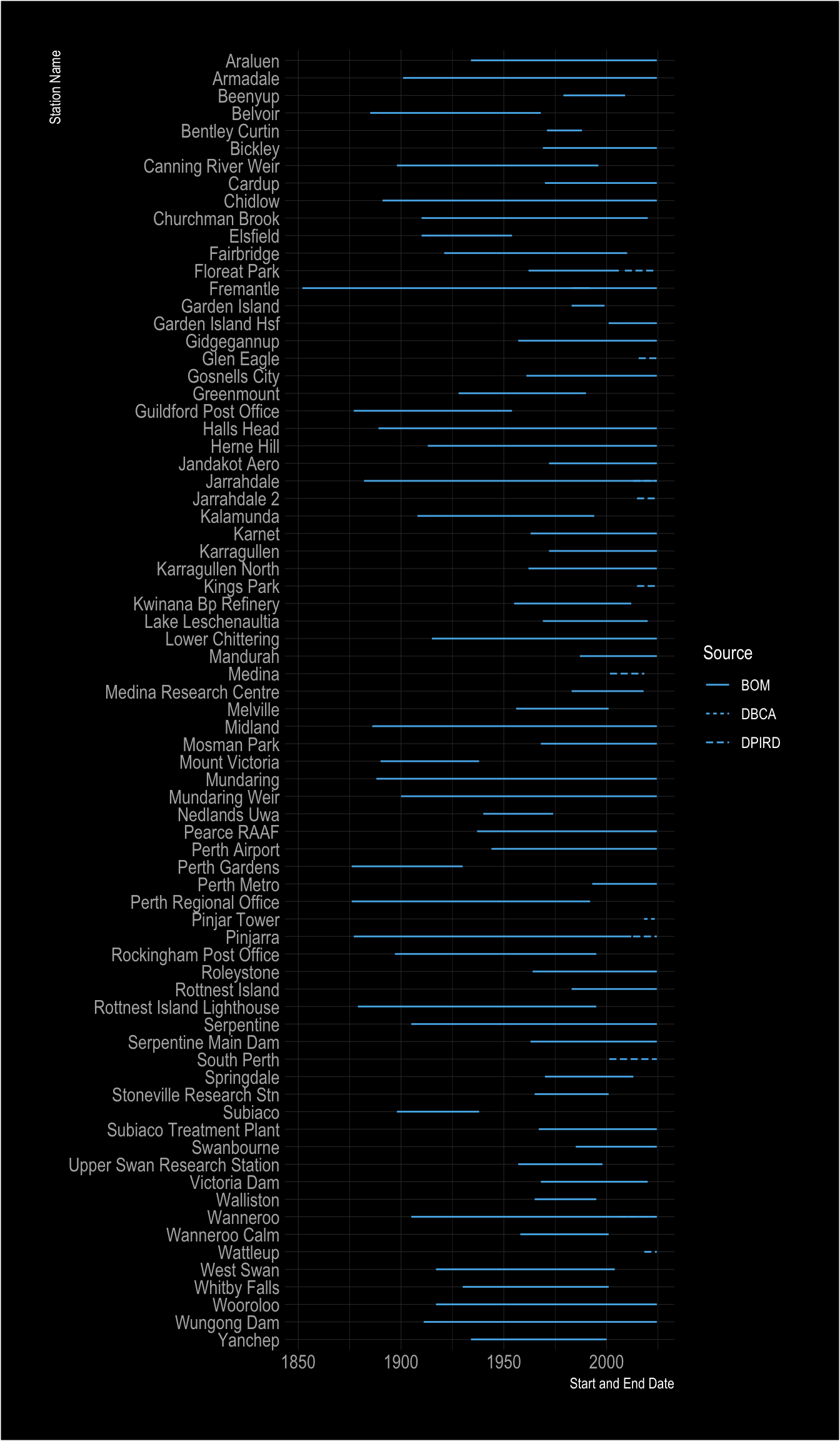
Visualise Station Availability
To visualise the data availability for the stations’ start and end dates, we will use {ggplot2} again.
|
|
Get Weather Data for Perth Stations
Using both the DPIRD and SILO APIs we can get weather from the mid-1800s to current.
Get DPIRD Stations’ Data
We will start with the DPIRD and DPIRD-hosted station data by creating a vector of station_code values for stations that are NOT BOM stations using subset() and then use droplevels() to drop unused factor levels from the vector.
|
|
There can be some hiccups when querying station data.
It’s a good idea to wrap it in a tryCatch() or something like purrr::possibly().
I’m a fan of using possibly() for these sorts of issues.
It makes it easy to spot stations with errors and investigate, but more importantly, it means you can use purrr::map(), lapply() or a for loop and if there is an error, you get the message you have specified and the operation carries on with the rest of the stations rather than stopping.
|
|
Now we will fill the list with weather data for the stations located in Greater Perth in the DPIRD network.
|
|
##              Length Class      Mode
## Floreat Park 9      data.table list
## Glen Eagle   9      data.table list
## Jarrahdale   9      data.table list
## Jarrahdale 2 9      data.table list
## Kings Park   9      data.table list
## Medina       9      data.table list
## Pinjar Tower 9      data.table list
## Pinjarra     9      data.table list
## South Perth  9      data.table list
## Wanneroo     9      data.table list
## Wattleup     9      data.table list
Next, bind the list into a single data frame object using data.table::rbindlist().
|
|
##
## Attaching package: 'data.table'

## The following object is masked from 'package:purrr':
##
##     transpose
|
|
Get BOM Stations’ Data
|
|
Following the same method as with the DPIRD station network, use possibly() to ensure that there are no interruptions when fetching data.
|
|
Now we will fill the list with weather data for the stations located in Greater Perth in the BOM network.
|
|
##                             Length Class      Mode
## Araluen                     12     data.table list
## Armadale                    12     data.table list
## Beenyup                     12     data.table list
## Belvoir                      1     -none-     character
## Bentley Curtin              12     data.table list
## Bickley                     12     data.table list
## Canning River Weir          12     data.table list
## Cardup                      12     data.table list
## Chidlow                     12     data.table list
## Churchman Brook             12     data.table list
## Elsfield                    12     data.table list
## Fairbridge                  12     data.table list
## Floreat Park                12     data.table list
## Fremantle                    1     -none-     character
## Fremantle                   12     data.table list
## Garden Island               12     data.table list
## Garden Island Hsf           12     data.table list
## Gidgegannup                 12     data.table list
## Gosnells City               12     data.table list
## Greenmount                  12     data.table list
## Guildford Post Office        1     -none-     character
## Halls Head                  12     data.table list
## Herne Hill                  12     data.table list
## Jandakot Aero               12     data.table list
## Jarrahdale                   1     -none-     character
## Kalamunda                   12     data.table list
## Karnet                      12     data.table list
## Karragullen                 12     data.table list
## Karragullen North           12     data.table list
## Kwinana Bp Refinery         12     data.table list
## Lake Leschenaultia          12     data.table list
## Lower Chittering            12     data.table list
## Mandurah                    12     data.table list
## Mandurah                    12     data.table list
## Medina Research Centre      12     data.table list
## Melville                    12     data.table list
## Midland                      1     -none-     character
## Mosman Park                 12     data.table list
## Mount Victoria              12     data.table list
## Mundaring                    1     -none-     character
## Mundaring Weir              12     data.table list
## Nedlands Uwa                12     data.table list
## Pearce RAAF                 12     data.table list
## Perth Airport               12     data.table list
## Perth Gardens                1     -none-     character
## Perth Metro                 12     data.table list
## Perth Regional Office        1     -none-     character
## Pinjarra                     1     -none-     character
## Rockingham Post Office      12     data.table list
## Roleystone                  12     data.table list
## Rottnest Island             12     data.table list
## Rottnest Island Lighthouse   1     -none-     character
## Serpentine                  12     data.table list
## Serpentine Main Dam         12     data.table list
## Springdale                  12     data.table list
## Stoneville Research Stn     12     data.table list
## Subiaco                     12     data.table list
## Subiaco Treatment Plant     12     data.table list
## Swanbourne                  12     data.table list
## Upper Swan Research Station 12     data.table list
## Victoria Dam                12     data.table list
## Walliston                   12     data.table list
## Wanneroo                    12     data.table list
## Wanneroo Calm               12     data.table list
## West Swan                   12     data.table list
## Whitby Falls                12     data.table list
## Wooroloo                    12     data.table list
## Wungong Dam                 12     data.table list
## Yanchep                     12     data.table list
Unsurprisingly there were a few issues along the way.
As there are a few stations with issues, I’ve chosen to use grep() to locate the faulty stations and drop them from the list while binding it into a single data fram object.
|
|
Create Data Set for Plotting
Now that we have clean sets of data we can bind the two sets of data.
{weatherOz} intentionally sets the column names to be the same, regardless of the API queried to make this easy to do.
Using data.table::bindrows() option, fill = TRUE makes this easier than dropping columns that are not shared.
|
|
##   station_code     station_name         longitude        latitude
##  009572 :  49467   Length:1454932     Min.   :115.5   Min.   :-32.70
##  009007 :  48737   Class :character   1st Qu.:115.8   1st Qu.:-32.22
##  009031 :  45450   Mode  :character   Median :116.0   Median :-32.03
##  009001 :  45085                      Mean   :116.0   Mean   :-32.05
##  009039 :  43624                      3rd Qu.:116.1   3rd Qu.:-31.86
##  009105 :  43624                      Max.   :116.3   Max.   :-31.56
##  (Other):1178945
##       year          month            day             date
##  Min.   :1889   Min.   : 1.00   Min.   : 1.00   Min.   :1889-01-01
##  1st Qu.:1952   1st Qu.: 4.00   1st Qu.: 8.00   1st Qu.:1952-08-14
##  Median :1980   Median : 7.00   Median :16.00   Median :1980-04-19
##  Mean   :1975   Mean   : 6.51   Mean   :15.73   Mean   :1975-02-12
##  3rd Qu.:2000   3rd Qu.:10.00   3rd Qu.:23.00   3rd Qu.:2000-09-19
##  Max.   :2024   Max.   :12.00   Max.   :31.00   Max.   :2024-06-09
##
##     air_tmax     air_tmax_source    elev_m            extracted
##  Min.   : 7.60   Min.   : 0.00   Length:1454932     Min.   :2024-06-09
##  1st Qu.:18.50   1st Qu.:25.00   Class :character   1st Qu.:2024-06-09
##  Median :22.50   Median :25.00   Mode  :character   Median :2024-06-09
##  Mean   :23.59   Mean   :23.95                      Mean   :2024-06-09
##  3rd Qu.:28.00   3rd Qu.:35.00                      3rd Qu.:2024-06-09
##  Max.   :50.90   Max.   :75.00                      Max.   :2024-06-09
##  NA's   :100     NA's   :49232                      NA's   :49232
Surprisingly, there are a few NA values in the data, so we will drop those.
|
|
##   station_code     station_name         longitude        latitude
##  009572 :  49467   Length:1454832     Min.   :115.5   Min.   :-32.70
##  009007 :  48737   Class :character   1st Qu.:115.8   1st Qu.:-32.22
##  009031 :  45450   Mode  :character   Median :116.0   Median :-32.03
##  009001 :  45085                      Mean   :116.0   Mean   :-32.06
##  009039 :  43624                      3rd Qu.:116.1   3rd Qu.:-31.86
##  009105 :  43624                      Max.   :116.3   Max.   :-31.56
##  (Other):1178845
##       year          month            day             date
##  Min.   :1889   Min.   : 1.00   Min.   : 1.00   Min.   :1889-01-01
##  1st Qu.:1952   1st Qu.: 4.00   1st Qu.: 8.00   1st Qu.:1952-08-13
##  Median :1980   Median : 7.00   Median :16.00   Median :1980-04-18
##  Mean   :1975   Mean   : 6.51   Mean   :15.73   Mean   :1975-02-11
##  3rd Qu.:2000   3rd Qu.:10.00   3rd Qu.:23.00   3rd Qu.:2000-09-17
##  Max.   :2024   Max.   :12.00   Max.   :31.00   Max.   :2024-06-09
##
##     air_tmax     air_tmax_source    elev_m            extracted
##  Min.   : 7.60   Min.   : 0.00   Length:1454832     Min.   :2024-06-09
##  1st Qu.:18.50   1st Qu.:25.00   Class :character   1st Qu.:2024-06-09
##  Median :22.50   Median :25.00   Mode  :character   Median :2024-06-09
##  Mean   :23.59   Mean   :23.95                      Mean   :2024-06-09
##  3rd Qu.:28.00   3rd Qu.:35.00                      3rd Qu.:2024-06-09
##  Max.   :50.90   Max.   :75.00                      Max.   :2024-06-09
##                  NA's   :49132                      NA's   :49132
We are only interested in the month of May, so we will remove all the other months’ data by selecting only May (month = 5).
|
|
Now we need to find the highest May temperatures for each station of each year.
Using .SD from {data.table}, we get this.
|
|
Next, create the annual mean.
|
|
Plotting May High Temperatures
Now we have a good data set for plotting.
Using {ggplot2} we can plot the high temperature for each station in May in light grey in the background with the mean stations’ maximum temperatures in the foreground. We can use {ggiraph} to make the plot interactive, similar to the ABC’s interactive version but with the extra data and greater ability to see the data points of all the stations each year.
|
|
Obviously, this data does not match ABC’s exactly, it does go back farther into the 1800s, 1852, with the inclusion of Fremantle and likely has more data in the more recent years with the inclusion of the DPIRD network data. Still, it is a fun exercise to work through getting the data, subsetting it and visualising.
-
Actually this function only now exists because I wanted to write this blog post and needed to find stations in the Perth metro area. ↩︎